Scapy is a utility that allows you to forge, receive and send packets or data frames over a network for a multitude of protocols. In this introduction, you'll discover this Python utility that enables traffic capture, network mapping, ARP cache poisoning, VLAN hopping, or passive operating system fingerprinting.
Scapy is a program developed in Python by Philippe Biondi (EADS CCR); it notably allows you to forge, receive and transmit packets and/or data frames via a network to or from an IT infrastructure for a multitude of different network protocols (IP, TCP, UDP, ARP, SNMP, ICMP, DNS, DHCP, ...) with precision and speed.
Scapy comes in the form of a single Python script file - 13,342 lines of code for version 1.1.1 that we'll use throughout this document. Among other notable features of Scapy, we'll note its ability to dissect packets and/or data frames as well as decode certain protocols.
Furthermore, Scapy can also perform network traffic monitoring and capture similar to reading pcap format captures from another traffic analyzer like Wireshark, for example.
It's also possible with Scapy to generate graphs in 2D and/or 3D from packets and/or data frames, or even port scanning like NMAP and passive remote operating system recognition like p0f.
According to its author, Scapy is capable by itself of replacing all of the following utilities: hping, 85% of NMAP, arpspoof, arp-sk, arping, tcpdump, tethereal, p0f and many other system commands (traceroute, ping, route, ...).
For the equivalent of about sixty lines of C code, the combination of Python and Scapy only requires a few lines most of the time to perform these different packet and/or data frame manipulation operations, resulting in considerable time savings for anyone who needs to perform this type of manipulation on a network.
For this, Scapy has many pre-defined functions allowing you to configure the injection of a packet (or frame) into a given network connection; some special functions of Scapy thus make it possible to perform common attacks with great simplicity (non-exhaustive list): network infrastructure mapping, ARP Cache Poisoning, Smurfing, VLAN Hopping as well as IP spoofing and rogue DHCP server setup.
These attacks can be combined with each other (ARP Cache Poisoning + VLAN Hopping for example) to perform security audits specifically adapted to the infrastructure in place whose security level you want to verify.
You can just as well intercept VOIP communications (packet/frame decoding) and this even on a WEP encrypted WIFI wireless connection as long as you know the decryption key associated with these connections (knowing of course that WEP is still secure).
This encryption key can be configured in Scapy, still provided that you have it, so that Scapy can use it during packet or data frame injection operations into the traffic of a WEP-encrypted wireless network (see also the WIFITAP utility developed by Cédric Blancher [EADS CCR] for traffic injection into WIFI connections).
Installation and configuration
This section concerns the installation of Scapy as well as all the elements necessary for its proper functioning on a GNU/LINUX system. It also includes Scapy's internal configuration system as a first approach to the utility as well as the different network configurations necessary for its use for the rest of this document.
Let's perform the preliminary installation necessary for using Scapy on a Debian/Ubuntu-like Linux operating system:
Now we configure the network interfaces present on the operating system of the machine that we are using for all the tests in this document; this information will help better understand the different tests we will be performing:
The section above needs to be adapted to each machine configuration depending on the network interfaces present; for the next part we test that network connectivity is working properly:
That's it, our machine with IP address 192.168.0.2 is able to ping the machine with IP address 192.168.0.1; we can now proceed to install Scapy by first downloading it:
If we want to get information about the configuration of the Scapy version we're using, simply type conf and press Enter to validate and execute the command:
Scapy also allows us to choose to view only part of the configuration if we want, here we want to display only information related to the routing table using the conf.route command:
The routing tables between the system and Scapy are different because Scapy has its own internal routing table.
We delete this entry with the conf.route.delt command, still for the 192.168.1.0/24 network with a machine acting as gateway whose IP address is 192.168.0.1:
Indeed, the entry is no longer present in the internal routing table; if we had wanted to add a route only to a particular machine, we could have used the following syntax (host= instead of net=) to specify that packets/frames destined for the machine whose IP address is 192.168.1.3 must be routed to the machine whose IP is 192.168.0.1, which thus acts as a gateway to access it:
The system is now fully functional, and we can move on to the packet/data frame manipulation functions offered by Scapy.
Basic Usage
This part of the Scapy documentation proposes to give an overview of the basic commands available in Scapy. It also includes different examples of their use that will allow you to become familiar with the internal functioning of this tool in order to better understand its principles.
First, we list all the protocols supported by Scapy using the ls() command:
As we can see, the number of supported protocols is quite substantial; each of these protocols has its own specifications that we can list using the ls() command. Here are the details of the ICMP protocol:
To display the documentation for a particular function, simply add the .doc extension behind the command (without the final ()); so to display the documentation for the arping() command, it will be necessary to type the following syntax:
>>>arping.__doc__
'Send ARP who-has requests to determine which hosts are up\narping(net, [cache=0,] [iface=conf.iface,] [verbose=conf.verb]) -> None\nSet cache=True if you want arping to modify internal ARP-Cache'
It's also possible to get the same documentation result but with a bit more layout using the lsc() command that allowed us to list the available commands in Scapy earlier; just add the name of the command in parentheses that you want documentation for:
Scapy can function like a network traffic analyzer to capture data for later viewing. This part of the documentation offers different examples of captures as well as the many ways available internally to view the results of these captures.
We display the documentation for the sniff() function using the lsc() function:
>>>sniff(filter="udp and host 192.168.0.2",count=30)<Sniffed:UDP:30ICMP:0TCP:0Other:0>
The 30 packets have been collected for the UDP protocol and the machine whose IP address is 192.168.0.2; we can view the results related to this capture by assigning the records to the variable sn via the variable _ in the following way:
If we want to view all these records contained in the variable sn, we need to add .nsummary() after the name of the variable that we chose when assigning the results of a function (here the sniff function and the sn variable):
Sn is considered here as an object in its own right on which we can apply different operations via appropriate functions like nsummary() here; to view in detail the first record contained in the variable sn, we need to add between [] the number of the record that we want to view in the traffic we just captured and this just behind the name of the variable:
With Scapy, we can also capture network traffic and directly display the results while specifying the network interface on which we want to perform this operation if of course it was different from the one defined in the conf.iface variable; this is done as follows:
We can also view the records in a completely different way by replacing the x.summary() attribute with the x.show() attribute, which this time will allow us to get much more intrinsic details about the traffic collected during the network capture; since the output can be quite long, we'll limit the number of packets we'll capture to 3 with count:
In the same way, we can capture network traffic for a given port or several given ports; here we capture the traffic (5 records) related to port 22 (usually equivalent to encrypted remote connection traffic like SSH) and port 80, which is usually synonymous with traffic to a web server like Apache (or IIS):
>>>sniff(filter="tcp and ( port 22 or port 80 )",prn=lambdax:x.sprintf("IP Source: %IP.src% ; Port Source: %TCP.sport% ---> IP Destination: %IP.dst% ; Port Destination: %TCP.dport% ; TCP Flags: %TCP.flags% ; Payload: %TCP.payload%"),count=5)IPSource:127.0.0.1;PortSource:33917--->IPDestination:127.0.0.1;PortDestination:ssh;TCPFlags:FA;Payload:
IPSource:127.0.0.1;PortSource:33917--->IPDestination:127.0.0.1;PortDestination:ssh;TCPFlags:FA;Payload:
IPSource:127.0.0.1;PortSource:ssh--->IPDestination:127.0.0.1;PortDestination:33917;TCPFlags:R;Payload:
IPSource:127.0.0.1;PortSource:ssh--->IPDestination:127.0.0.1;PortDestination:33917;TCPFlags:R;Payload:
IPSource:127.0.0.1;PortSource:33917--->IPDestination:127.0.0.1;PortDestination:ssh;TCPFlags:FA;Payload:
<Sniffed:UDP:0TCP:5ICMP:0Other:0>
The x.sprintf attribute in the example above allows you to format the output results of Scapy's functions according to your preferences using pre-defined variables such as %IP.src% for the source IP address, %IP.dst% for the destination IP address, %TCP.sport% for the TCP source port, %TCP.dport% for the TCP destination port as well as %TCP.flags% for the options activated in the TCP flags as well as %TCP.payload% for the useful payload related to the record being viewed.
The use of these variables and their manipulation accentuate the object-oriented side of the Scapy utility; for example, we can display the information related to a record in the following way:
>>>IP(dst="192.168.0.2")<IPdst=192.168.0.2|>
>>>a.sprintf("IP Source %IP.src% ; IP Destination %IP.dst% ; TTL %IP.ttl%")'IP Source 192.168.0.2 ; IP Destination 192.168.0.2 ; TTL 64'
Note that even if we didn't specify values for the ttl, Scapy takes a default value equivalent to 64 that we find when displaying via the %IP.ttl% variable.
The sequence of commands that will follow presents itself in the form of a capture of traffic equivalent to ports 22 (SSH) and/or 80 (WWW) for a total of 5 records related to the TCP transport protocol; the collected records will be stored in a variable sn for which we can display the first record with sn[0]:
>>>sniff(filter="tcp and ( port 22 or port 80 )",count=5)<Sniffed:UDP:0ICMP:0TCP:5Other:0>
>>>sn=_
>>>sn[0]<Etherdst=00:00:00:00:00:00src=00:00:00:00:00:00type=0x800|<IPversion=4Lihl=5Ltos=0x0len=60id=45016flags=DFfrag=0Lttl=64proto=tcpchksum=0x8ce1src=127.0.0.1dst=127.0.0.1options=''|<TCPsport=56283dport=sshseq=2821237960Lack=0dataofs=10Lreserved=0Lflags=Swindow=32792chksum=0x5b8aurgptr=0options=[('MSS',16396),('SAckOK',''),('Timestamp',(1180432,0)),('NOP',None),('WScale',5)]|>>>
This sequence of commands can also be written in an even more simplified way as follows:
>>>sn=sniff(filter="tcp and ( port 22 or port 80 )",count=5)>>>sn[0]<Etherdst=00:00:00:00:00:00src=00:00:00:00:00:00type=0x800|<IPversion=4Lihl=5Ltos=0x0len=60id=35250flags=DFfrag=0Lttl=64proto=tcpchksum=0xb307src=127.0.0.1dst=127.0.0.1options=''|<TCPsport=56788dport=sshseq=2937645191Lack=0dataofs=10Lreserved=0Lflags=Swindow=32792chksum=0xb8bcurgptr=0options=[('MSS',16396),('SAckOK',''),('Timestamp',(1204533,0)),('NOP',None),('WScale',5)]|>>>
Traceroute and 2D/3D Visualization
Through different examples of traceroutes performed using Scapy, we'll discover the graphical functionalities of Scapy to generate two and three-dimensional graphs from the results of these traceroutes. You'll also see the different ways you can export these results for visualization.
We now display the information related to Scapy's traceroute command:
We then perform a simple traceroute to define the path taken by network traffic to go from the test machine to the IP address associated at the DNS level to the FQDN (Full Qualified Domain Name) and this with a latency time equal to 10 jiffies (number of clock periods); recall that TCP/IP networks are fragmentation and packet-switched networks, so it's normal to find a different packet routing result between two traceroutes launched at different intervals:
We then perform a multiple traceroute to the FQDNs "www.free.fr" and "www.exoscan.net" with a ttl still equal to 10; the results are stored in the variable sn for records that had a response while those without a response are stored in the variable unans:
The multiple traceroute results are stored in the sn variable for records representing a response; we can just as well display the content of the sn variable in the following way using the show() attribute:
We can similarly view the records contained in the sn variable by placing the nsummary() attribute instead of the show() attribute for the following result:
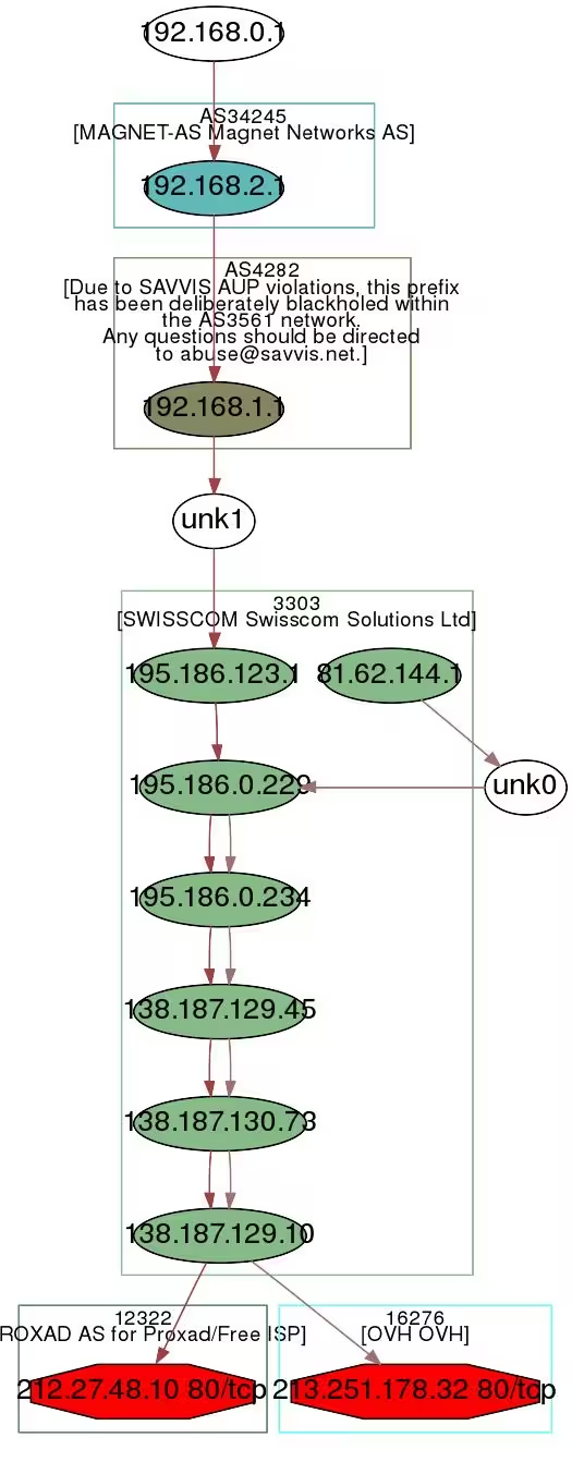
We launch a new multiple traceroute but this time just to the FQDNs "www.free.fr" and "www.secuobs.com" with a ttl still equal to 10, the positive responses are still stored in the sn variable while the records without response go into the unans variable (for unanswered):
From these results and using the graph() attribute, we can generate a graph of the routing taken by the data flows to reach these two different destinations from the test machine used for this document:
We can observe on the graph below these different routing results:
We could also have saved the generated graph directly to an image file in our operating system's file system (here in the /tmp directory for an svg image format and an image file named graph.svg):
We can also directly print these graphs provided that a printer is connected to the machine and configured at the operating system level allowing it to function (here a postscript type printer):
The vpython visual plugin we're using here allows you to zoom on this graph using the 3rd mouse button; if this button is emulated, simply press the left and right mouse or touchpad buttons simultaneously. You can also move the graphical representation with the left mouse button and tilt it with the right button:
This time we'll perform a multiple traceroute to the FQDNs "www.free.fr", "www.google.fr" and "www.microsoft.com" with a ttl equivalent to 10; the responses are still stored in the sn variable while the records corresponding to no responses are contained in the unans variable:
We get the following result as a 3D graph of the results:
Packet and Frame Manipulation
Scapy is above all a utility for forging, receiving, and sending packets and frames of data over a network. This section covers the many functions available for this purpose through different examples such as performing an ICMP ping or a port scan.
We now display the specifications of the IP protocol using the ls() command:
We note with the sr1() function that we only receive and record one packet in response. This same function can also be used to perform a port scan; we send a TCP/IP packet to www.secuobs.com to port 80 with the TCP Syn flag activated which indicates that we are asking to establish a connection without preliminaries:
We note here that we received a packet in response, we can conclude that port 80 (www) is open on the server whose IP address is assigned to the FQDN "www.secuobs.com"; we make a second attempt on port 22 (SSH):
We conclude that port 53 is not open on this server, it doesn't necessarily mean that a DNS server isn't running on this port, we can just conclude that filtering rules are present to prevent external connections to this port 53.
We now display, using the lsc() command, the details of the options of the sr() function which allows it to receive and store more than one packet in response to those previously sent:
We can also use Scapy's srloop function to execute a loop on sending a data packet (here ICMP to the machine whose IP address is equal to 192.168.0.2):
Press Ctrl+C to stop srloop, here we have sent and received 9 packets; we can also assign to srloop() a limited send number with the count parameter, here 10 packets:
The functions sr, sr1, send and srloop send and/or receive packets at the network level, which is layer 3 of the OSI model, that is, the one present just before (emission) or after (reception) the level corresponding to the data link which is in second position in this 7-layer model.
The data link layer is therefore just before (emission) or after (reception) the level corresponding to the physical layer of the OSI model.
The equivalent of these network level functions for the data link level in Scapy are the functions srp, srp1, srploop and sendp which forge, receive and/or send data frames and not just data packets on the network; note that at the physical layer of the OSI model we speak in bytes and no longer in packets or data frames.
We could also have assigned certain values to the sending of the frame like the number of times they should be resent after a negative response thanks to the retry parameter (here 3 times), the time interval between the sending of two frames with inter (here 1) or the time limit (here 2) to wait after sending the last frame with timeout (all of these parameters also being available for sending packets via the sr() function):
Scapy provides great flexibility in handling the various commands available. It's thus possible to manage each field of a packet or a function in the manner of an object that can be defined in a variable and then represented and visualized in several ways.
>>>_.display()###[ IP ]###version=4L
ihl=5L
tos=0x0
len=135id=13021flags=frag=0L
ttl=62proto=udp
chksum=0x3a95
src=62.4.16.70
dst=192.168.0.2
options=''###[ UDP ]###sport=domain
dport=domain
len=115chksum=0x7504
###[ DNS ]###id=0qr=1L
opcode=QUERY
aa=0L
tc=0L
rd=1L
ra=1L
z=0L
rcode=ok
qdcount=1ancount=1nscount=2arcount=1\qd\|###[ DNS Question Record ]###|qname='exoscan.net.'|qtype=A
|qclass=IN
\an\|###[ DNS Resource Record ]###|rrname='exoscan.net.'|type=A
|rclass=IN
|ttl=3469|rdlen=0|rdata='213.186.41.29'\ns\|###[ DNS Resource Record ]###|rrname='exoscan.net.'|type=NS
|rclass=IN
|ttl=28243|rdlen=0|rdata='ns7.gandi.net.'|###[ DNS Resource Record ]###|rrname='exoscan.net.'|type=NS
|rclass=IN
|ttl=28243|rdlen=0|rdata='custom2.gandi.net.'\ar\|###[ DNS Resource Record ]###|rrname='ns7.gandi.net.'|type=A
|rclass=IN
|ttl=643|rdlen=0|rdata='217.70.177.44'
We now launch a capture on all traffic, still using the sniff() command, asking to capture only one record (still with the count option) which we will place as usual in the sn variable:
As we've already noted previously, Scapy follows an object orientation by offering significant flexibility in the operations of manipulating the different functions that are present there but also in the parameters and attributes that refer to these functions; we now display again the specifications of the IP protocol using the ls() command:
Each field of a packet or frame can also be considered as an object and its value can then be defined by a variable just as it is possible to do in the same way for parts or sub-parts of functions and this with a direct rebound effect on the values (of these fields) that were defined by default:
As we just saw by changing the values of the variables a.dst and a.ttl the modifications are directly impacted on the variable a and the values of the ttl and dst parameters are replaced by the changes made or they are simply deleted in the same way as the parameter when it has been previously deleted.
The different parameters of the function however return to default values when deleted as we can see with the value of a.dst which is equal to 127.0.0.1 in the end or that of a.ttl which is equivalent to 64.
In Scapy we can also generate a representation of a packet and/or frame type object with the str function whose specifications are as follows:
We now generate an Ethernet frame (level 2 data link layer in the OSI model for the TCP/IP protocol suite) corresponding to this packet which coupled the IP() and TCP() functions and now the Ether() function:
Note that all fields with a default value are visible, it's possible to remove them with the hide*default() attribute applied to the current result * (or to a variable):
This part of the Scapy documentation allows you to find all the web addresses related to this documentation and to the use of Scapy. It also includes an example of a custom tool developed using Scapy and the Python language, in our case a TCP port scanner.
You can find different PDF slides about Scapy including those from the PacSec Core05 conference, Hack.lu 2005, Summerschool Applied IT Security 2005, T2 2005, CanSecWest Core05 and LSM 2003.
For users of Microsoft Windows operating systems, you can get the Windows port of Scapy (while OpenBSD system users can read this document for installation).
If you want to create specific scripts with Scapy, you can consult the document provided for this purpose on the official Scapy website, SecDev.org. For example, if you want to create a TCP port scanner, the corresponding Python script should look more or less like this (here for ports 22 to 25 inclusive):
#!/usr/bin/env pythonimportsysfromscapyimport*target=sys.argv[1]fl=22while(fl<=25):p=sr1(IP(dst=target)/TCP(dport=fl,flags="S"),retry=0,timeout=1)ifp:print"\n Port "+str(fl)+" TCP is open on "+str(target)+"\n"else:print"\n Port "+str(fl)+" TCP is not open on "+str(target)+"\n"fl=fl+1
We save this script under the name scan.py (note that the file must be in the same directory as the scapy.py file) which we will run with the Python interpreter by passing the IP address or FQDN of the machine we want to define as the target of the port scan as follows:
#!/usr/bin/env pythonimportsysfromscapyimport*target=sys.argv[1]fl=1while(fl<=1024):p=sr1(IP(dst=target)/TCP(dport=fl,flags="S"),retry=0,timeout=1)ifp:print"\n Port "+str(fl)+" TCP is open on "+str(target)+"\n"else:print"\n Port "+str(fl)+" TCP is not open on "+str(target)+"\n"fl=fl+1
Given the number of ports to test and the length of the result, it's preferable to launch it in the following way:
Note that it may be necessary to adjust the timeout value in the line "p=sr1(IP(dst=target)/TCP(dport=fl, flags="S"),retry=0,timeout=1)" depending on the locations of the different machines present (source and destination) in order to obtain satisfactory results.
A whole chapter dedicated to Scapy was written by the author himself, Philippe Biondi; this chapter is published in the book Security Power Tools; 856 pages published by O'Reilly Media (ISBN-10: 0596009631; ISBN-13 978-0596009632).